Published: Jan 15, 2023 by Jacob Young
We introduce the design ideas of an AAIS from the viewpoint of a device provider. In this tutorial, we briefly discuss superconducting machines with fixed-frequency transmon qubits and present how to build an AAIS based on these machines.
Superconducting Qubits
Superconducting circuits are a promising platform for scalable quantum computing. Carefully constructed mesoscopic circuits can be designed to have quantum behavior, allowing easier exploitation of quantum effects for quantum computation. A simple superconducting LC oscillator can be quantized in terms of the phase and charge moving within the circuit, and by replacing the inductor with a Josephson Junction, a component serving as a nonlinear inductor, the oscillator becomes anharmonic, separating out the lower two energy levels of the oscillation to use as the computational basis of a qubit. Treating each oscillator as a two-level system yields the approximate qubit Hamiltonian \(H = \omega_q \frac{\sigma_z}{2}\), where \(\omega_q\) is the oscillation frequency of the qubit’s precession about the z-axis. When constructed with certain circuit parameters, this simple anharmonic oscillator is known as a transmon qubit.
Superconducting Qubit Control
Qubit control is accomplished through the use of signal lines, dedicated signal paths where arbitrary waveform generators can modify the Hamiltonian of the qubit(s) affected by that line. For a single qubit drive line, in the frame of reference rotating with the qubit, the qubit has no system Hamiltonian, and the Hamiltonian induced by a pulse applied to the drive line may be written as \(H_d = g_d s(t) (\cos(\theta) \sigma_x + \sin(\theta) \sigma_y)\), where \(g_d\) and \(s(t)\) are the interaction strength and signal envelope for the applied pulse and \(\theta\) is the phase of the pulse. We emphasize that to produce this Hamiltonian in the rotating frame, in the lab frame, pulses are constructed with a frequency matching that of the qubit.
This format for single-qubit drive operations gives rise to an important feature of superconducting qubits– the free Z rotation. The phase of the drive signal relative to the qubit determines whether an X or Y rotation is performed– the same thing accomplished by rotating a qubit about its Z axis. Furthermore, because measurements are performed in the Z basis, the global phase of a given qubit is irrelevant. Updating the phase used when sending drive signals to the qubit is equivalent to performing a single-qubit Z rotation. Tracking this phase shift in software instead of driving the qubit allows for instantaneous, parametrized, error-free Z rotations.
For multi-qubit entangling lines, two coupled fixed-frequency transmon qubits are entangled through the cross-resonance interaction. This interaction is induced by driving one qubit at the other qubit’s frequency, resulting in a Hamiltonian of the form \(H_{CR} = g_{CR} s(t) (\nu \sigma_x \otimes I + \mu I \otimes \sigma_x + \sigma_z \otimes \sigma_x)\), where \(g_{CR}\), \(\nu\), and \(\mu\) are interaction strength constants, \(s(t)\) is the signal envelope, and the tensor product indicates Hamiltonian terms affecting both systems. A ZX polyrotation may be extracted from this Hamiltonian through the careful application of multiple drive signals on both qubits, resulting in an effective Hamiltonian of \(H_{eff} = g_{CR} \sigma_z \otimes \sigma_x\).
Initializing the Machine and Extracting Backend Details
We begin by creating a machine object with some number of qubits– in this case, 27. We build our machine with a call to QMachine() and add qubits to it with calls to qubit(mach).
mach = QMachine()
n = 27
ql = [qubit(mach) for i in range(n)]
We can extract qubit coupling information directly from the IBM backend targeted by our AAIS.
IBMQ.load_account()

provider = IBMQ.get_provider(hub=<your_hub>, group=<your_group>, project=<your_project>)
backend = provider.get_backend(<27_qubit_ibm_backend>)

control_line_by_system = {tuple(v['operates']['qubits']): int(k.strip("u")) for k, v in backend.configuration().channels.items() if v['purpose'] == 'cross-resonance'}

link = list(self.control_line_by_system.keys())
print("New list of connected pairs for IBM system: " + str(link))
Building Single-Qubit Signal Lines
For each qubit on our machine, we build a single-qubit X-Y drive interaction in the format described above, and we define a derived Z instruction implemented in software via the free Z interaction. Each signal line is built and added to the machine with a call to SignalLine(mach), and each instruction is built with a call to Instruction(<Signal_Line>, <Instruction_Type>, <Instruction_Label>). We define the instruction Hamiltonians term by term intuitively using SimuQ Expressions and assign them with calls to instruction.set_ham(<Expression>). Note that instructions have two types– native and derived– corresponding to Hamiltonians that can be created more directly on the processor and instructions whose effective Hamiltonians are formed from some combination of effects. The SimuQ compiler treats these types differently, allowing native instructions on different lines affecting the same systems to be executed simultaneously. By contrast, derived instructions may inherently involve operations on other lines and are not scheduled simultaneously with other instructions affecting the same systems. As described earlier, the X_Y instruction is directly supported and therefore native, whereas the the software-implemented free Z rotation is considered a derived instruction.
for i in range(n) :
    L = SignalLine(mach)

    ins1 = Instruction(L, 'native', 'L{}_X_Y'.format(i))
    amp = LocalVar(ins1)
    phase = LocalVar(ins1)
    ins1.set_ham(amp * (Expression.cos(phase) * ql[i].X + Expression.sin(phase) * ql[i].Y))

    ins2 = Instruction(L, 'derived', 'L{}_Z'.format(i))
    amp = LocalVar(ins2)
    ins2.set_ham(amp * ql[i].Z)
Building Multi-Qubit Signal Lines
We iterate through the coupled pairs identified earlier and build an entangling signal line for each pair. Here, because of the complexity involved in extracting the ZX polyrotation from the Cross-Resonance Hamiltonian, all instructions are considered derived instructions. Furthermore, the underlying hardware may perform a change of basis operation to convert the ZX polyrotation into other basic polyrotations, allowing us to easily support additional instructions. Note that in our SimuQ Expressions, multiplication of two operators on different qubits corresponds to taking the tensor product of the two operators
for (q0, q1) in link :
    L = SignalLine(mach)

    ins = Instruction(L, 'derived', 'L{}{}_ZX'.format(q0, q1))
    amp = LocalVar(ins)
    ins.set_ham(amp * ql[q0].Z * ql[q1].X)

    ins = Instruction(L, 'derived', 'L{}{}_XX'.format(q0, q1))
    amp = LocalVar(ins)
    ins.set_ham(amp * ql[q0].X * ql[q1].X)

    ins = Instruction(L, 'derived', 'L{}{}_YY'.format(q0, q1))
    amp = LocalVar(ins)
    ins.set_ham(amp * ql[q0].Y * ql[q1].Y)

    ins = Instruction(L, 'derived', 'L{}{}_ZZ'.format(q0, q1))
    amp = LocalVar(ins)
    ins.set_ham(amp * ql[q0].Z * ql[q1].Z)