Published: Jan 30, 2023 by Yuxiang Peng
We introduce the design ideas of AAIS from the viewpoint of a device provider. In this tutorial, we briefly discuss the Rydberg atom arrays and present how to build an AAIS for them.
Rydberg atom arrays
A Rydberg atom array is typically made by Yb or Rb atoms. Optical tweezers are utilized to trap neutral atoms on a 2-D plane (there are devices support placing in 3-D space). The placement of the atoms normally has restrictions like limited square region and lower bounds of atom distances. In this introduction, we neglect these restrictions for simplicity.
The atoms have multiple energy levels and scientists particularly chose the minimal energe state as \(\vert 0\rangle\) (or \(\vert g\rangle\)) and a high energy state as \(\vert 1\rangle\) (or \(\vert r\rangle\)) called the Rydberg state. There exist other hyperfine states while we do not use them in this note.
Assume the positions of the atoms are \(\{(x_j, y_j)\}\) (unit: \(\mu m\)). Between two atoms indexed by \(j\) and \(k\), there is an interaction called van der Waals force attracting the two atoms. The effect of this force can be expressed as \(\frac{C_6}{d^6(j, k)}\hat{n}_j\hat{n}_k.\) Here \(d(j, k)=\sqrt{(x_j-x_k)^2+(y_j-y_k)^2}\) is the distance between them, \(\hat{n}_j\) is the number operator of the atom \(j\), and \(C_6\) is the Rydberg interaction constant. Most current devices do not support moving atoms after experiment set-up.
The atoms are driven by laser beams targeting them. Current QuEra devices have global laser control: all atoms are targetted by the same laser beam configuration. Future Rydberg atom array devices may have local laser control: the laser configurations are customizable for different atoms. For the \(j\)-th laser targeting atom \(j\), there are three independent configurable parameters: detuning \(\Delta_j\), amplitude \(\Omega_j\), and phase \(\phi_j\). These parameters are real functions of time. The effect of this laser beam is characterized by Hamiltonian \(-\Delta_j\hat{n}_j+\frac{\Omega_j}{2}(\cos(\phi_j)X_j-\sin(\phi_j)Y_j).\) Here \(X_j, Y_j, Z_j\) are the Pauli operators and \(\hat{n}_j=(I_j-Z_j)/2\) are the number operators for qubits.
We create a quantum environment for a 2-D Rydberg atom array with local laser control. Assume that we have n atoms.
Rydberg = QMachine()
q = [qubit(Rydberg) for i in range(n)]
Global variables and system Hamiltonian
We model the positions of atoms as global variables in the AAIS, because it is only configurable before the start of the experiment and keeps the same during the experiment. We create a list of global variables by the following Python code
x = [(0, 0)] + [(GlobalVar(Rydberg), GlobalVar(Rydberg)) for i in range(1, n)]
The first element of x is set to (0, 0) to reduce the degree of freedom. You can also set initial value used in the solver here, by specifying init_value in the definition of GlobalVar. Since the default initial value is 0 for variables, it may cause numerical issues for van der Waals forces. We recommend initial values by heuristics from your target problem.
The van der Waals interactions between each pair of atoms is then determined by x. Since these interactions can not be neglected or turned off, we model them as the system Hamiltonian, which is always on when synthesizing Hamiltonian. The following code calculates the summation of these effects.
noper = [(q[i].I - q[i].Z) / 2 for i in range(n)]
sys_h = 0
for i in range(n) :
    for j in range(i) :
        dsqr = (x[i][0] - x[j][0])**2 + (x[i][1] - x[j][1])**2
        sys_h += (C6 / (dsqr ** 3)) * noper[i] * noper[j]
Rydberg.set_sys_ham(sys_h)
The algebraic expressions above defining noper make use of SimuQ Expression, and is intuitive when being read. They represent the number operators $\hat{n}$. The following nested loops enumerate atom pairs and calculate the van der Waals effects between the atoms in the pair. The command set_sys_ham then sets the system Hamiltonian of Rydberg.
Signal lines, instructions and local variables
Signal lines are abstraction of signal carriers of the machine. On our Rydberg machines, the signal carriers are the laser beams. We hence define a signal line for each laser beam.
L = [SignalLine(Rydberg) for i in range(n)]
We directly create an instruction for each signal line to package the effect of the laser beam. Three local variables are defined to represent the three configurable parameters of a laser beam.
for i in range(n) :
    ins = Instruction(L[i], 'native')
    d, o, p = LocalVar(ins), LocalVar(ins), LocalVar(ins)
    ins.set_ham(- d * noper[i] + o / 2 * (cos(p) * q[i].X - sin(p) * q[i].Y))
Here the property of this instruction is native, meaning that the effect of this instruction is direct and can apply simultaneously with other native instructions (including the system Hamiltonian). This is because the laser beam’s effect is directly built in the instruction, and multiple laser beams’ effects can present at the same time.